Examples of A priori models¶

Multiple 1D Gaussian prior model¶

A prior model consisting of three independent 1D distributions (a Gaussian, Laplace, and Uniform distribution) can be defined using

ip=1;
prior{ip}.type='GAUSSIAN';
prior{ip}.name='Gaussian';
prior{ip}.m0=10;
prior{ip}.std=2;

ip=2;
prior{ip}.type='GAUSSIAN';
prior{ip}.name='Laplace';
prior{ip}.m0=10;
prior{ip}.std=2;
prior{ip}.norm=1;

ip=3;
prior{ip}.type='GAUSSIAN';
prior{ip}.name='Uniform';
prior{ip}.m0=10;
prior{ip}.std=2;
prior{ip}.norm=60;

m=sippi_prior(prior);

m =

    [14.3082]    [9.4436]    [10.8294]

1D histograms of a sample (consisting of 1000 realizations) of the prior models can be visualized using …

sippi_plot_prior_sample(prior);

## Multivariate Gaussian prior with unknown covariance model properties.¶

The FFT-MA type a priori model allow separation of properties of the covariance model (covariance parameters, such as range, and anisotropy ratio) and the random component of a Gaussian model. This allow one to define a Gaussian a priori model, where the covariance parameters can be treated as unknown variables.

In order to treat the covariance parameters as unknowns, one must define one a priori model of type FFTMA, and then a number of 1D GAUSSIAN type a priori models, one for each covariance parameter. Each gaussian type prior model must have a descriptive name, corresponding to the covariance parameter that is should describe:

prior{im}.type='gaussian';
prior{im}.name='m_0';     % to define a prior for the mean
prior{im}.name='sill';    % to define a prior for sill (variance)
prior{im}.name='range_1'; % to define a prior for the range parameter 1
prior{im}.name='range_2'; % to define a prior for the range parameter 2
prior{im}.name='range_3'; % to define a prior for the range parameter 3
prior{im}.name='ang_1';   % to define a prior for the first angle of rotation
prior{im}.name='ang_2';   % to define a prior for the second angle of rotation
prior{im}.name='ang_3';   % to define a prior for the third angle of rotation
prior{im}.name='nu';      % to define a prior for the shape parameter, nu
              %   (only applies when the Matern type Covariance model is used)

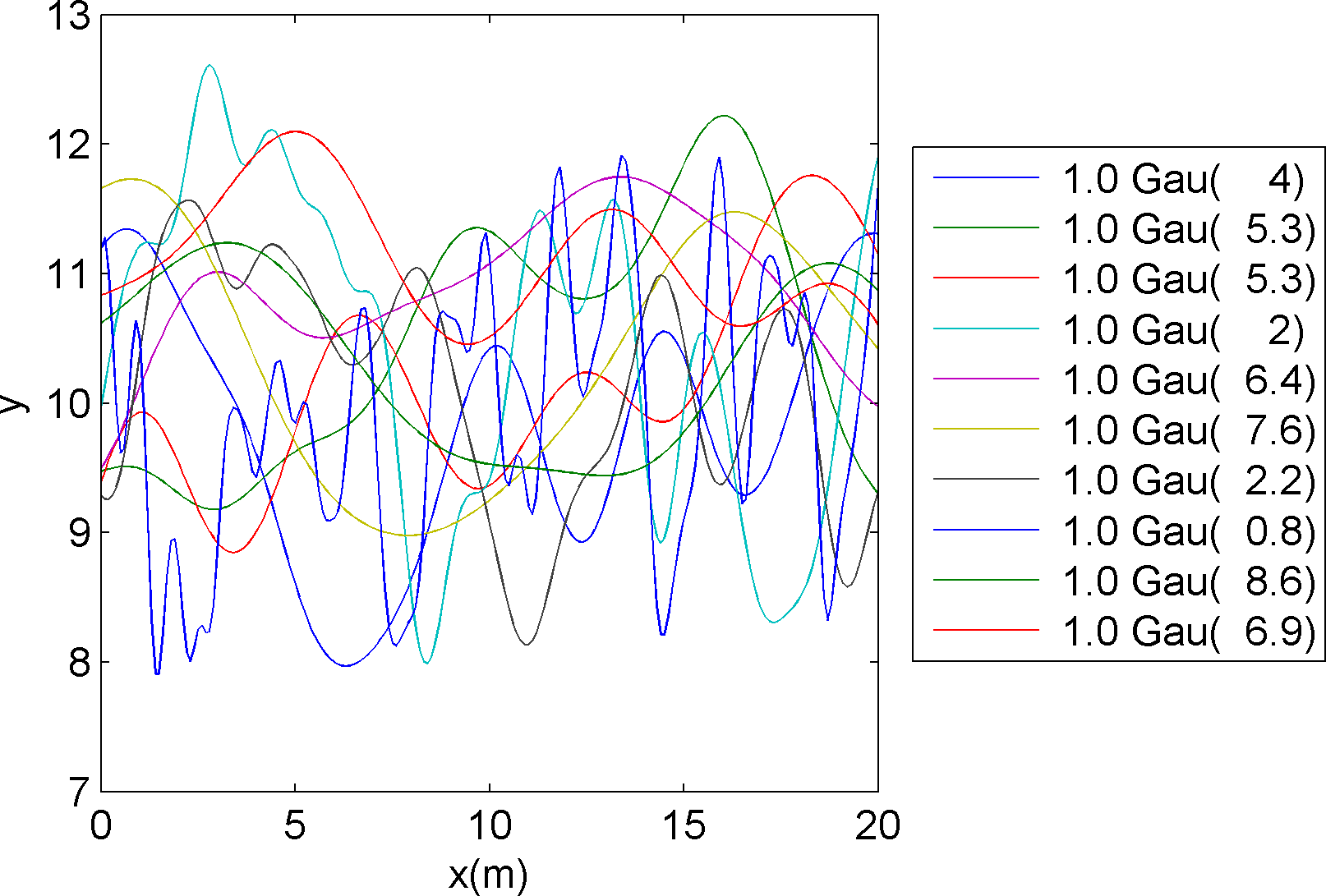
A very simple example of a prior model defining a 1D Spherical type covariance model with a range between 5 and 15 meters, can be defined using:

im=1;
prior{im}.type='FFTMA';
prior{im}.x=[0:.1:10]; % X array
prior{im}.m0=10;
prior{im}.Va='1 Sph(10)';
prior{im}.fftma_options.constant_C=0;


im=2;
prior{im}.type='gaussian';
prior{im}.name='range_1';
prior{im}.m0=10;
prior{im}.std=5
prior{im}.norm=80;
prior{im}.prior_master=1; % -- NOTE, set this to the FFT-MA type prior for which this prior type
                          % should describe the range

Note that the the field prior_master must be set to point the to the FFT-MA type a priori model (through its id/number) for which it should define a covariance parameter (in this case the range).

10 independent realizations of this type of a priori model are shown in the following figure

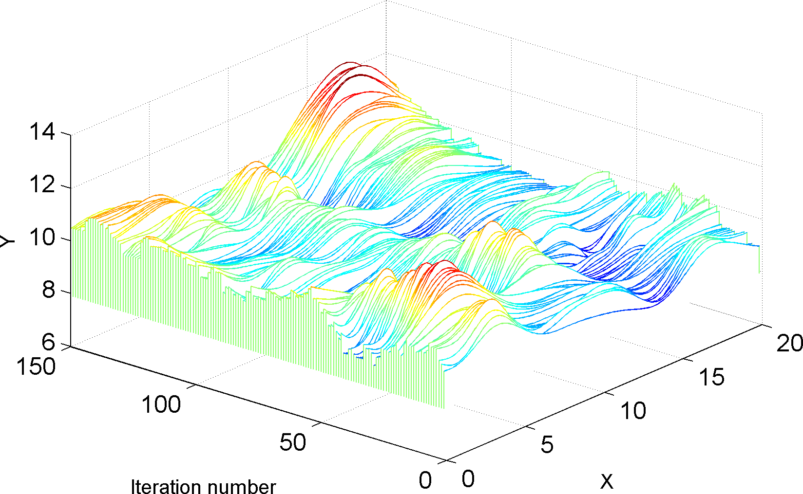
Such a prior, as all prior models available in SIPPI, works with sequential Gibbs sampling, allowing a random walk in the space of a prior acceptable models, that will sample the prior model. An example of such a random walk can be performed using

prior{1}.seq_gibbs.step=.005;
prior{2}.seq_gibbs.step=0.1;
clear m_real;
for i=1:150;
    [m,prior]=sippi_prior(prior,m);
    m_real(:,i)=m{1};
end

An example of such a set of 150 dependent realization of the prior can be seen below

Unknown

Simulating the cover of Joy Division’s Unknown Pleasers¶

SIPPI can be used to simulate something similar to the iconic cover of Joy Divisions’s Unknown Pleasures.

%% Setup two prior structuresx=linspace(0.1,.9,101);d_target=rand(1,1000);
nl=60; % number of lines

ip=1;
prior{ip}.type='FFTMA';
prior{ip}.x=x;
prior{ip}.y=1:1:nl;
prior{ip}.m0=0;
prior{ip}.Va='0.1 Sph(.1,90,0.001)';
prior{ip}.d_target=d_target/20;

ip=2;
prior{ip}.type='FFTMA';
prior{ip}.x=x;
prior{ip}.y=1:1:nl;
prior{ip}.m0=0;
prior{ip}.Va='.99 Gau(.06,90,0.001) + .01 Sph(.1,90,0.001)';
prior{ip}.d_target=3*d_target;

%% Compute a padding matrix, such that prior{2} is only used 'in the middle' pad=zeros(size(x));
x1=0.3;ix1=find(x>=x1);
ix1=min(ix1);x2=0.4;
ix2=find(x>=x2);ix2=ix2(1);xx1=ix1:1:ix2;
fadein=sin(interp1([ix1 ix2],[0 pi/2],xx1));
pad(find(x>x1&x<(1-x2)))=1;
pad(xx1)=fadein;

xx2=fliplr(length(x)-xx1);
pad(xx2)=fliplr(fadein);

% add a small fading from left to rightlinpad=linspace(1.3,0.0,length(x));pad=pad.*linpad;

pad=repmat(pad,nl,1);

%% Generate first realization.[m,prior]=sippi_prior(prior);
mm=m{1}+m{2}.*pad;

mm will now contain one realizations that when visualized should look similar to the original album cover. A movie of a random walk in this ‘prior’ model obtained using sequential Gibbs sampling can now be performed, and will render something similar to this video: {% youtube %}https://www.youtube.com/watch?v=La0uESBYLEA{% endyoutube %}

The full source is available at SIPPI/examples/prior_tests/unknown_pleasures.m