FFTMA - 3D Gaussian model
The FFT moving average method provides an efficient approach for computing unconditional realizations of a Gaussian random field.
The mean and the covariance model must be specified in the m0 and
Cm fields. The format for describing the covariance model follows
‘gstat’ notation, and is described in more details in the mGstat
manual.
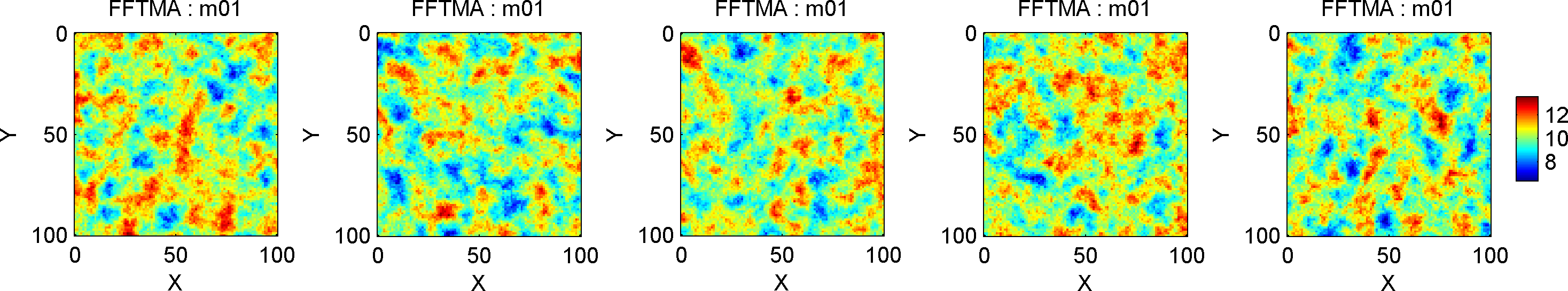
A 2D covariance model with mean 10, and a Spherical type covariance model can be defined in a 101x101 size grid (1 unit (e.g., meters) between the cells) using
im=1;
prior{im}.type='FFTMA';
prior{im}.x=[0:1:100];
prior{im}.y=[0:1:100];
prior{im}.m0=10;
prior{im}.Cm='1 Sph(10)';
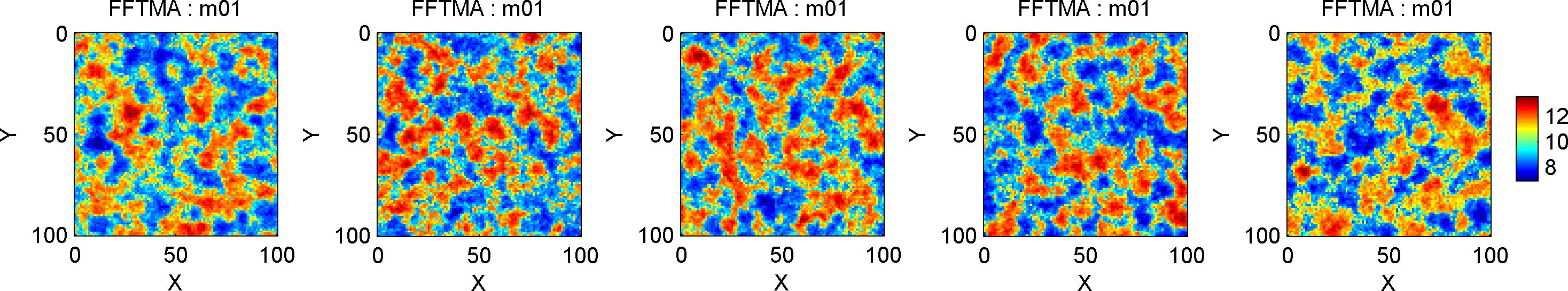
Optionally one can translate the output of the Gaussian simulation into an arbitrarily shaped ‘target’ distribution, using normal score transformation. Note that this transformation will ensure a certain 1D distribution of the model parameters to be reproduced, but will alter the assumed covariance model such that the properties of covariance model are not necessarily reproduced. To ensure that both the covariance model properties and the 1D distribution are reproduced, make use of the VISIM type prior model instead because it utilizes direct sequential simulation.
im=1;
prior{im}.type='FFTMA';
prior{im}.x=[0:1:100];
prior{im}.y=[0:1:100];
prior{im}.Cm='1 Sph(10)';

% Create target distribution
N=10000;
prob_chan=0.5;
d1=randn(1,ceil(N*(1-prob_chan)))*.5+8.5;
d2=randn(1,ceil(N*(prob_chan)))*.5+11.5;
d_target=[d1(:);d2(:)];
prior{im}.d_target=d_target;
prior{im}.m0=0; % to make sure no trend model is assumed.
Alternatively, the normal score transformation can be defined manually such that the tail behavior can be controlled:
N=10000;
prob_chan=0.5;
d1=randn(1,ceil(N*(1-prob_chan)))*.5+8.5;
d2=randn(1,ceil(N*(prob_chan)))*.5+11.5;
d_target=[d1(:);d2(:)];
[d_nscore,o_nscore]=nscore(d_target,1,1,min(d_target),max(d_target),0);
prior{im}.o_nscore=o_nscore;
FFTMA - 3D Gaussian model with variable covariance model properties
The FFTMA method also allows treating the parameters defining the Gaussian model, such as the mean, variance, ranges and angles of rotation as a priori model parameters (that can be inferred as part of inversion, see e.g. an example).
First a prior type defining the Gaussian model must be defined (exactly as listed above):
im=im+1;
prior{im}.type='FFTMA';
prior{im}.x=[0:.1:10]; % X array
prior{im}.y=[0:.1:20]; % Y array
prior{im}.m0=10;
prior{im}.Cm='1 Sph(10,90,.25)';
Now, all parameter such as the mean, variance, ranges and angles of
rotations, can be randomized by defining a 1D a priori model type
(‘uniform’ or ‘gaussian’), and with a specific ‘name’ indicating the
parameter (see this example for a
complete list of names), and by assigning the prior_master field
that points the prior model id for which the parameters should
randomized.
For example the range along the direction of maximum continuty can be
randomized by defining a prior entry named ‘range_1’, and settting the
prior_master to point to the prior with id 1:
im=2;
prior{im}.type='uniform';
prior{im}.name='range_1';
prior{im}.min=2;
prior{im}.max=14;
prior{im}.prior_master=1;
I this case the range is randomized following a uniform distribution U[2,14].
Likewise, the first angle of rotation can be randomized using for example
im=3;
prior{im}.type='gaussian';
prior{im}.name='ang_1';
prior{im}.m0=90;
prior{im}.std=10;
prior{im}.prior_master=1;
A sample from such a prior type model will thus show variability also in the range and angle of rotation, as seen here